The Math Behind a Neural Network
Understanding neural networks requires diving into their mathematical foundation. At its core, every neural network operates on a fundamental principle of weighted summation followed by non-linear transformation:
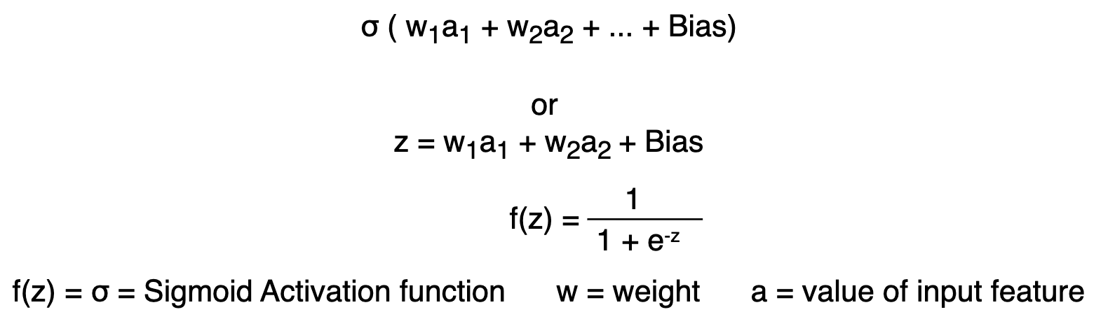
Each neuron processes information by combining weighted inputs with a bias term, then applying an activation function to introduce non-linearity (example with Sigmoid-Function). This seemingly simple operation becomes incredibly powerful when scaled across multiple layers and neurons.
Medical Dataset: PSA Levels and Cancer Detection
To illustrate these concepts, we'll work with a medical dataset focused on cancer prediction using PSA (Prostate-Specific Antigen) levels. PSA is a protein produced by the prostate gland, and elevated levels can indicate potential prostate cancer. Our goal is to build a neural network that can classify patients as healthy or at-risk based on their PSA measurements:
| Status | PSA Level |
|---|---|
| Cancer | 3.8 |
| Cancer | 3.4 |
| Cancer | 2.9 |
| Cancer | 2.8 |
| Cancer | 2.7 |
| Cancer | 2.1 |
| Cancer | 1.6 |
| Healthy | 2.5 |
| Healthy | 2.0 |
| Healthy | 1.7 |
| Healthy | 1.4 |
| Healthy | 1.2 |
| Healthy | 0.9 |
| Healthy | 0.8 |
Building Our First Neural Network
For our initial approach, we'll construct a minimal neural network architecture: a single input neuron receiving PSA values, directly connected to two output neurons representing the probability distribution between healthy and cancer classifications. This direct mapping, while simple, demonstrates the core mechanics of neural computation.
Through iterative training on our dataset, the network learns optimal connection weights. The resulting trained architecture appears as follows:
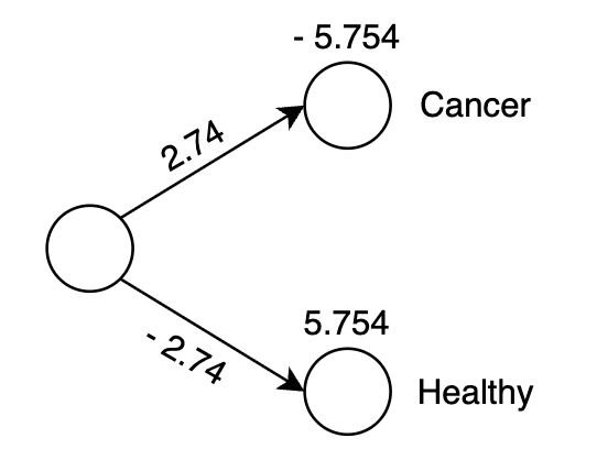
To validate our model's performance, we'll test it with a PSA level of 2.0—a value that, according to our training data, should indicate a healthy patient:

The network outputs a 43% probability for cancer, which translates to a 57% probability for the healthy classification. Since 57% > 43%, our model correctly predicts this patient as healthy, aligning with the expected outcome from our training data.
The Learning Process: Optimizing Weights and Biases
The critical question becomes: how does the network discover these optimal weights and biases? This process involves comparing predictions against known outcomes and systematically reducing prediction errors.
Consider our PSA level of 2.0 example: while our model predicts 57% healthy, we know from the training data that this patient is definitively healthy (100% certainty). This discrepancy—predicted value of 0.57 versus actual value of 1.0—represents the error our network must learn to minimize.
By computing these prediction errors across all training samples, we can quantify the network's overall performance using a cost function. This mathematical tool measures how far our predictions deviate from reality:
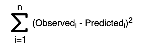
The cost function serves as our optimization target—the lower the cost, the better our model's performance. Through systematic adjustment of weights and biases, we can minimize this cost and improve prediction accuracy.
Introducing Complexity: A Network with Hidden Layers
While our initial model works, real-world problems often require more sophisticated architectures. Hidden layers enable networks to learn complex, non-linear relationships that simple direct connections cannot capture. Our enhanced architecture includes:
- Input Layer: Single neuron accepting PSA measurements
- Hidden Layer: One neuron with sigmoid activation for non-linear transformation
- Output Layer: Single neuron with sigmoid activation, producing probabilities between 0 and 1
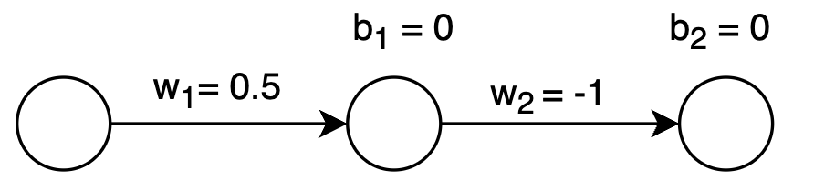
Neural networks begin their learning journey with randomly initialized parameters. For our demonstration, we'll start with these values:
w1 = 0.5      # connection strength: input → hidden layer
b1 = 0.0      # hidden layer bias term

w2 = -1.0     # connection strength: hidden → output layer
b2 = 0.0      # output layer bias term

Learning rate η = 0.1    # controls adaptation speed
The learning rate η = 0.1 represents a moderate pace of adjustment—large enough to make meaningful progress, yet small enough to avoid overshooting optimal solutions. Choosing the right learning rate balances training speed with stability.
Backpropagation: Learning from Mistakes
Backpropagation represents the heart of neural network learning—a systematic method for propagating errors backward through the network to update parameters. We'll trace through this process using our PSA level 2.0 example, where the target output should be 0 (healthy patient).
Forward Pass: Making a Prediction
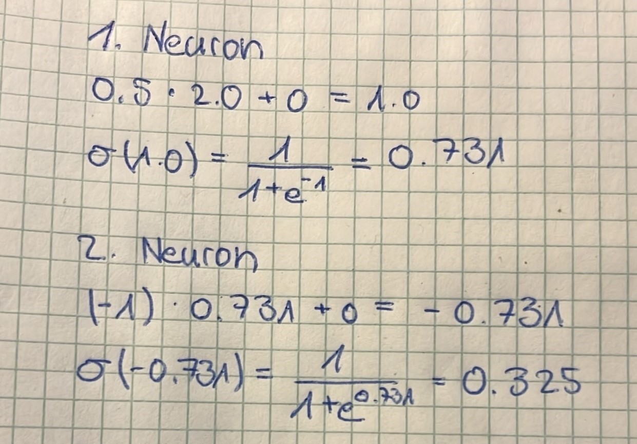
Our untrained network produces an output of 0.3248, which deviates from our target value of 0.
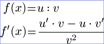
We quantify this error using the Sum of Squared Residuals (SSR) cost function. An alternative would be: Binary Cross-Entropy. The factor of ½ serves a practical purpose—it simplifies the derivative calculations during backpropagation:

The Chain Rule: Connecting Errors to Parameters
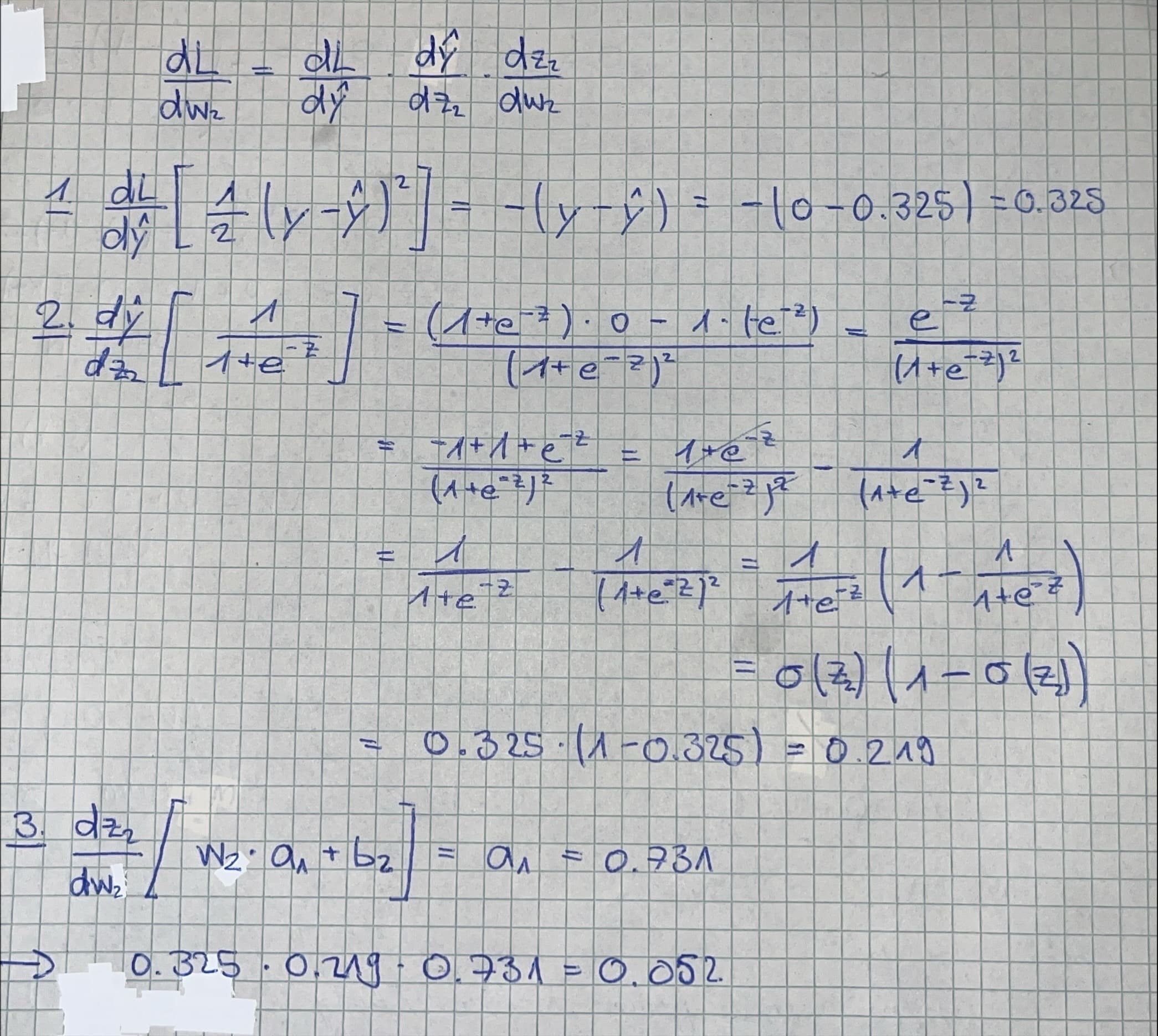
Backpropagation relies on the mathematical chain rule to trace how each parameter contributes to the final error. Since our network processes information through multiple layers, we cannot directly compute how changing a weight affects the output. Instead, we decompose this relationship into manageable steps:
The chain rule enables us to work backward from the error, layer by layer, computing gradients that indicate both the direction and magnitude of necessary parameter adjustments. Each gradient component tells us something specific about our network's behavior:
| Gradient Component | Mathematical Interpretation |
|---|---|
| dL / d𝑦 | Sensitivity of error (Loss function) to output changes |
| d𝑦 / dz₂ | Sigmoid activation function slope at output layer |
| dz₂ / dw₂ | Impact of output weight on pre-activation signal |
| dz₂ / da₁ | Connection pathway to hidden layer activations |
| da₁ / dz₁ | Hidden layer sigmoid gradient |
| dz₁ / dw₁ | Input weight influence on hidden layer |
Computing Parameter Gradients
Now we'll calculate specific gradients for each parameter, starting from the output layer and working backward through the network.
Output weight gradient (w₂): This determines how changes to the final connection affect our prediction error.
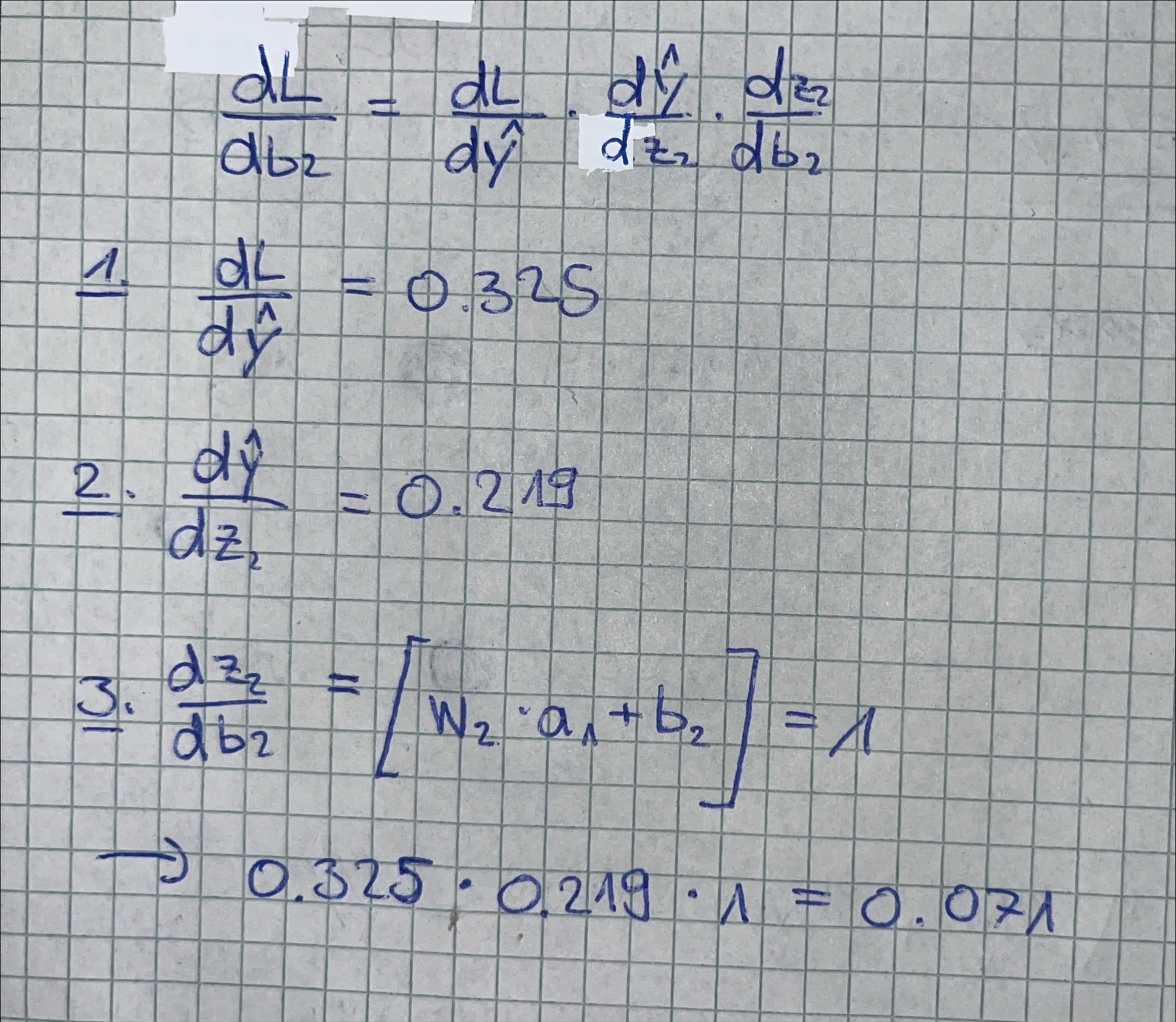
Output bias gradient (b₂): The bias provides a baseline adjustment independent of input magnitude.
Hidden weight gradient (w₁): This calculation requires propagating the error signal through the output layer to reach the hidden layer connection.
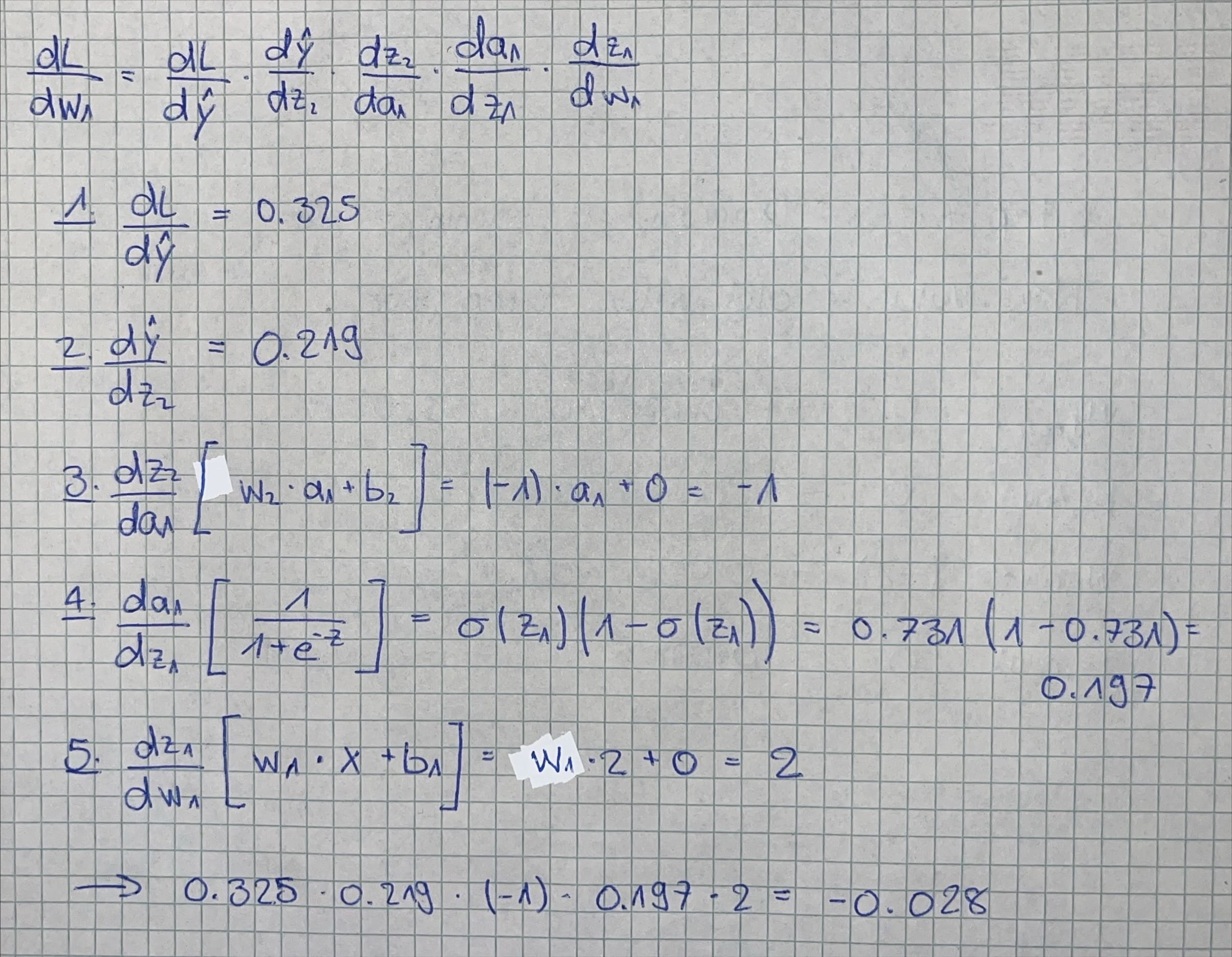
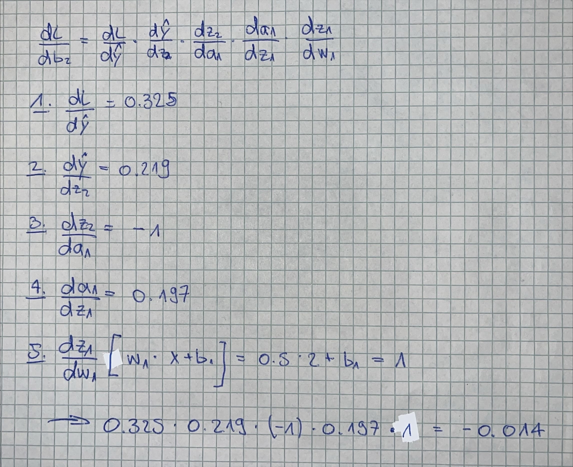
Hidden bias gradient (b₁): Similar to the hidden weight, but affecting the baseline activation of the hidden neuron.
Parameter Updates: Learning from Gradients
Armed with our computed gradients, we can now update each parameter using gradient descent. The learning rate η controls the step size—too large and we might overshoot the optimal solution, too small and learning becomes painfully slow:
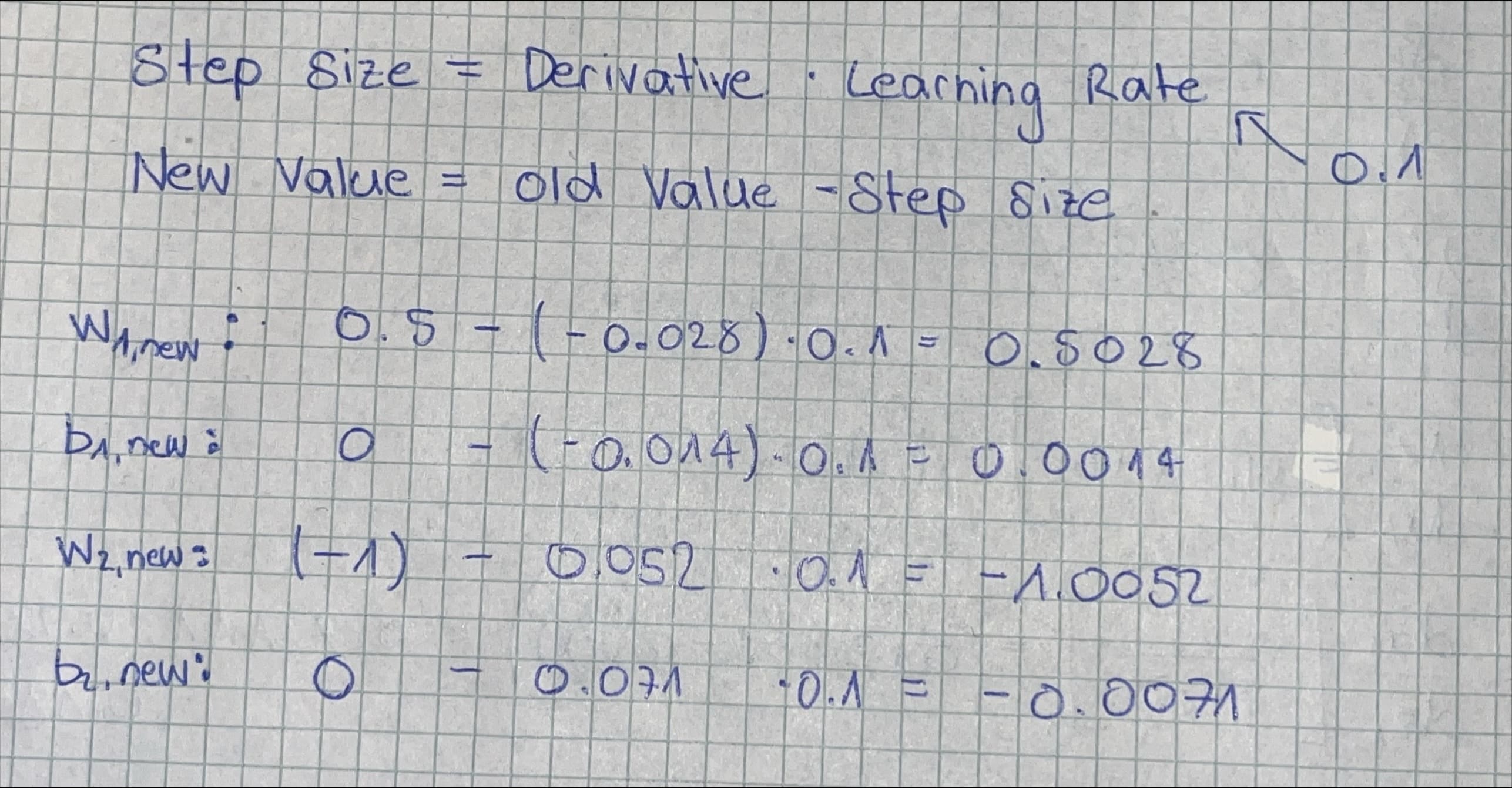
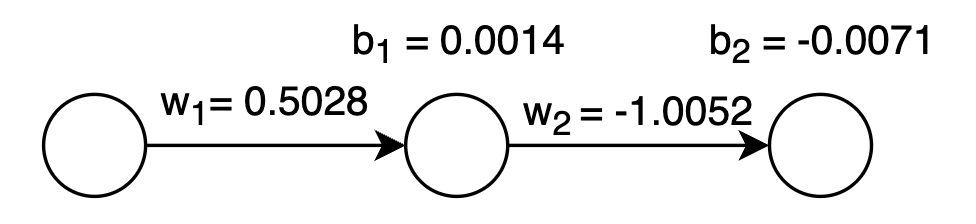
These updated parameters represent our network's first step toward better performance. The magnitude and direction of each update reflect how that parameter contributed to the prediction error.
To validate our parameter updates, we'll run another forward pass with PSA level 2.0. The updated network produces an output of 0.322, and when we calculate the SSR loss, we get 0.0519—a small improvement that demonstrates our backpropagation step worked as intended.
Scaling to Real-World Performance
The single training example we've examined represents just one iteration of the learning process. In practice, neural networks require exposure to the entire training dataset multiple times (called epochs) to achieve robust performance.
Each epoch involves processing every training sample, computing gradients, and updating parameters. Over many epochs, the network gradually adjusts its internal representation to minimize prediction errors across all training examples.
Continuous Improvement: I welcome feedback, corrections and clarity of these explanations. Machine learning is a rapidly evolving field, and collaborative refinement helps create better educational resources for everyone.
Acknowledgments: Special thanks to StatQuest for their excellent educational content. Check out their channel at https://www.youtube.com/@statquest